Random Matrix Theory
Zhiyu He, September 15, 2026
This note is adapted from the following sources:
- Tropp, J. A. (2015). An Introduction to Matrix Concentration Inequalities. Foundations and Trends in Machine Learning, 8(1–2), 1–230. doi & pdf
- Chen, Y. (2020). Matrix Concentration Inequalities. Lecture notes, Princeton University (ELE 520: Mathematics of High-Dimensional Data). pdf
1. What Is a Random Matrix, and Why Care?
A random matrix is a matrix whose entries are drawn at random — say a symmetric \(\mathbf{X} \in \mathbb{R}^{d \times d}\) with \(X_{ij} = X_{ji} \sim \mathcal{N}(0,1)\) independent and identically distributed. Classical random matrix theory asks what the spectrum of such a matrix looks like, and answers in the asymptotic regime when \(d \to \infty\), where the empirical eigenvalue distribution converges to a limiting spectral density.
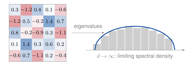
This tutorial takes a different route. Instead of examining one large matrix, we study a sum of independent random matrices,
\[\mathbf{S} = \sum_{k=1}^{n} \mathbf{X}_k \in \mathbb{R}^{d_1 \times d_2}, \qquad (\mathbf{X}_1, \ldots, \mathbf{X}_n) \ \text{independent},\]and we ask for finite-sample (non-asymptotic) guarantees — bounds that hold for every \(n\) and \(d\), not only in the limit.

The object of interest is the deviation of \(\mathbf{S}\) from its expectation \(\mathbb{E}[\mathbf{S}]\), measured in the spectral norm. The key question is
\[\mathbb{P}\left\{ \|\mathbf{S} - \mathbb{E}[\mathbf{S}]\| \geq t \right\} \leq \ \underline{\quad \textbf{?} \quad}\]There are three things to take away:
- Applications in statistics and machine learning;
- The setup and guarantee of the matrix Bernstein inequality;
- The proof for the basic case with a symmetric matrix.
2. The Relevance of the Independent Sum Model
Sample covariance estimation
Let \(\mathbf{x}_1, \ldots, \mathbf{x}_n \in \mathbb{R}^{d}\) be i.i.d., zero mean, with unknown covariance \(\mathbf{C} = \mathbb{E}[\mathbf{x} \mathbf{x}^*]\). The empirical covariance
\[\hat{\mathbf{C}}_n = \frac{1}{n} \sum_{k=1}^{n} \mathbf{x}_k \mathbf{x}_k^*, \qquad \mathbb{E}[\hat{\mathbf{C}}_n] = \mathbf{C},\]has error \(\hat{\mathbf{C}}_n - \mathbf{C} = \sum_{k=1}^{n} \mathbf{X}_k\) with \(\mathbf{X}_k = \tfrac{1}{n}(\mathbf{x}_k \mathbf{x}_k^* - \mathbf{C})\). This is an independent sum of centered matrices.
The question is how many samples guarantee \(\|\hat{\mathbf{C}}_n - \mathbf{C}\| \leq \varepsilon \|\mathbf{C}\|\)?
Least squares with random data
Given i.i.d. data \((\mathbf{a}_k, y_k)_{k=1}^{n}\), the empirical risk and its Hessian are
\[\hat{f}_n(\mathbf{x}) = \frac{1}{2n} \sum_{k=1}^{n} (\mathbf{a}_k^* \mathbf{x} - y_k)^2, \qquad \hat{\mathbf{H}}_n \triangleq \nabla^2 \hat{f}_n(\mathbf{x}) = \frac{1}{n} \sum_{k=1}^{n} \mathbf{a}_k \mathbf{a}_k^*.\]With the population Hessian \(\mathbf{H} = \mathbb{E}[\mathbf{a} \mathbf{a}^*]\) we again get \(\hat{\mathbf{H}}_n - \mathbf{H} = \sum_{k=1}^{n} \mathbf{X}_k\), \(\mathbf{X}_k = \tfrac{1}{n}(\mathbf{a}_k \mathbf{a}_k^* - \mathbf{H})\). Controlling this deviation means the empirical problem inherits the curvature of the population one.
How many samples ensure \(\|\hat{\mathbf{H}}_n - \mathbf{H}\| \leq \varepsilon \|\mathbf{H}\|\)?
Randomized matrix multiplication
Computing \(\mathbf{A} \mathbf{B}\) with \(\mathbf{A} \in \mathbb{R}^{d_1 \times N}\), \(\mathbf{B} \in \mathbb{R}^{N \times d_2}\) costs \(\mathcal{O}(N d_1 d_2)\). This operation can become prohibitive when the inner dimension \(N\) is huge. The column–row view
\[\mathbf{A} \mathbf{B} = \sum_{i=1}^{N} \mathbf{a}_i \mathbf{b}_i^*\]writes the product as a sum of \(N\) rank-one terms, so we may keep only \(n \ll N\) sampled terms.
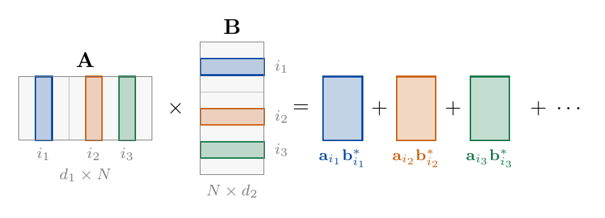
Sample indices \(i_1, \ldots, i_n\) i.i.d. with \(\mathbb{P}(i_k = j) = p_j\), then reweight to stay unbiased:
\[\mathbf{M}_{i_k} = \frac{1}{p_{i_k}} \mathbf{a}_{i_k} \mathbf{b}_{i_k}^*, \qquad \hat{\mathbf{M}}_n = \frac{1}{n} \sum_{k=1}^{n} \mathbf{M}_{i_k}, \qquad \mathbb{E}[\hat{\mathbf{M}}_n] = \mathbf{A} \mathbf{B}.\]This is once more an independent sum, now at cost \(\mathcal{O}(n d_1 d_2)\).
The question is again how many samples \(n \ll N\) suffice for a given accuracy?
The common structure
All three problems share the model \(\mathbf{S} = \sum_{k=1}^{n} \mathbf{X}_k\) with independent summands, and all three ask for \(\|\mathbf{S} - \mathbb{E}[\mathbf{S}]\|\) in spectral norm.
In the scalar case \(d_1 = d_2 = 1\) the answer is the classical Bernstein inequality, whose tail is driven by the variance \(\sum_k \operatorname{Var}(X_k)\); the matrix case needs a matrix analogue of that variance. The similar machinery extends beyond independence, e.g. to matrix martingales with \(\mathbb{E}[\mathbf{X}_{k+1} \mid \mathbf{X}_1, \ldots, \mathbf{X}_k] = \mathbf{X}_k\).
3. The Matrix Bernstein Inequality
Let \(\mathbf{X}_1, \ldots, \mathbf{X}_n \in \mathbb{R}^{d \times d}\) be independent and symmetric — they may follow different distributions — with
\[\mathbb{E}[\mathbf{X}_k] = \mathbf{0}, \qquad \|\mathbf{X}_k\| \leq B, \qquad v \triangleq \Big\|\mathbb{E}\Big[\sum_{k} \mathbf{X}_k^2\Big]\Big\|, \qquad \mathbf{S} = \sum_{k=1}^{n} \mathbf{X}_k.\]Matrix Bernstein (symmetric case). For all \(t \geq 0\),
\[\begin{align*} \mathbb{P}\{\lambda_{\max}(\mathbf{S}) &\geq t\} \leq d \exp\left(\frac{-t^2/2}{v + Bt/3}\right), \\ \mathbb{E}\, \lambda_{\max}(\mathbf{S}) &\leq \sqrt{2 v \log d} + \tfrac{1}{3} B \log d. \end{align*}\]
Two quantities shape the bound: the matrix variance statistic \(v\) and the problem dimension \(d\), the latter entering only logarithmically in expectation.
The bound interpolates between two tail behaviors, with the crossover at \(t \approx v/B\):
\[\mathbb{P}\{\lambda_{\max}(\mathbf{S}) \geq t\} \lesssim \begin{cases} d \exp\big(-t^2/(2v)\big), & t \ll v/B \quad \text{(Gaussian tail)} \\[.4em] d \exp\big(-t/B\big), & t \gg v/B \quad \text{(exponential tail)} \end{cases}\]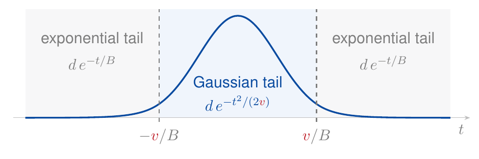
Small deviations are governed by the variance statistic \(v\); large deviations by the uniform bound \(B\).
4. Application: Randomized Matrix Multiplication
Return to \(\hat{\mathbf{M}}_n\) and choose the sampling probabilities proportional to squared norms,
\[p_j = \frac{\|\mathbf{a}_j\|^2 + \|\mathbf{b}_j\|^2}{\|\mathbf{A}\|_{\mathrm{F}}^2 + \|\mathbf{B}\|_{\mathrm{F}}^2}, \quad j = 1, \ldots, N,\]which costs only \(\mathcal{O}(N(d_1 + d_2))\) to form. Normalize \(\|\mathbf{A}\| = \|\mathbf{B}\| = 1\) and define the average stable rank
\[\operatorname{asr} \triangleq \tfrac{1}{2}\big(\operatorname{srank}(\mathbf{A}) + \operatorname{srank}(\mathbf{B})\big), \qquad \operatorname{srank}(\mathbf{X}) = \frac{\|\mathbf{X}\|_{\mathrm{F}}^2}{\|\mathbf{X}\|^2} \leq \operatorname{rank}(\mathbf{X}).\]The Bernstein parameters then satisfy \(\|\mathbf{M}_j\| \leq \operatorname{asr}\) and \(v(\mathbf{M}_j) \leq 2\operatorname{asr}\), so with \(d \triangleq d_1 + d_2\),
\[\mathbb{E}\,\|\hat{\mathbf{M}}_n - \mathbf{A} \mathbf{B}\| \leq \sqrt{\frac{4 \operatorname{asr} \log d}{n}} + \frac{2 \operatorname{asr} \log d}{3 n}.\]Consequently \(n \geq \varepsilon^{-2} \cdot \operatorname{asr} \cdot \log d\) samples give \(\mathbb{E}\|\hat{\mathbf{M}}_n - \mathbf{A}\mathbf{B}\| \leq 2\varepsilon + \tfrac{2}{3}\varepsilon^2\). The stable rank replaces the inner dimension \(N\), for a total cost \(\mathcal{O}(\varepsilon^{-2} \operatorname{asr} d_1 d_2 \log d)\).
Numerical experiments
Take \(\mathbf{A} \in \mathbb{R}^{80 \times 4000}\) and \(\mathbf{B} \in \mathbb{R}^{4000 \times 60}\) with \(\|\mathbf{A}\| = \|\mathbf{B}\| = 1\) and \(d = 140\). Here \(\operatorname{srank}(\mathbf{A}) = \operatorname{srank}(\mathbf{B}) = 9.6\), so \(\operatorname{asr} = 9.6 \ll N = 4000\) — the regime where sampling pays off. Each trial draws \(n\) index pairs with \(p_j \propto \|\mathbf{a}_j\|^2 + \|\mathbf{b}_j\|^2\), reweights by \(1/(n p_j)\), and averages.
Try it yourself: fill in rand_matmul(A, B, n, p, rng) and run the code in Google Colab.
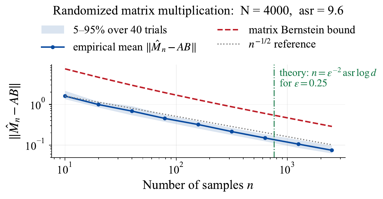
The estimation error follows the predicted \(n^{-1/2}\) rate; the bound is loose only in the constant.
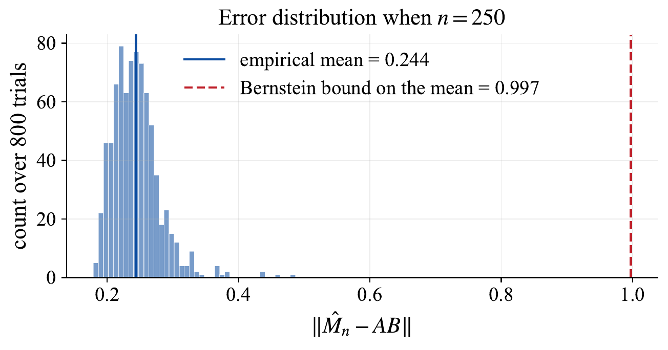
Across 800 trials at \(n = 250\), the error is sharply concentrated — exactly what a matrix concentration inequality promises.
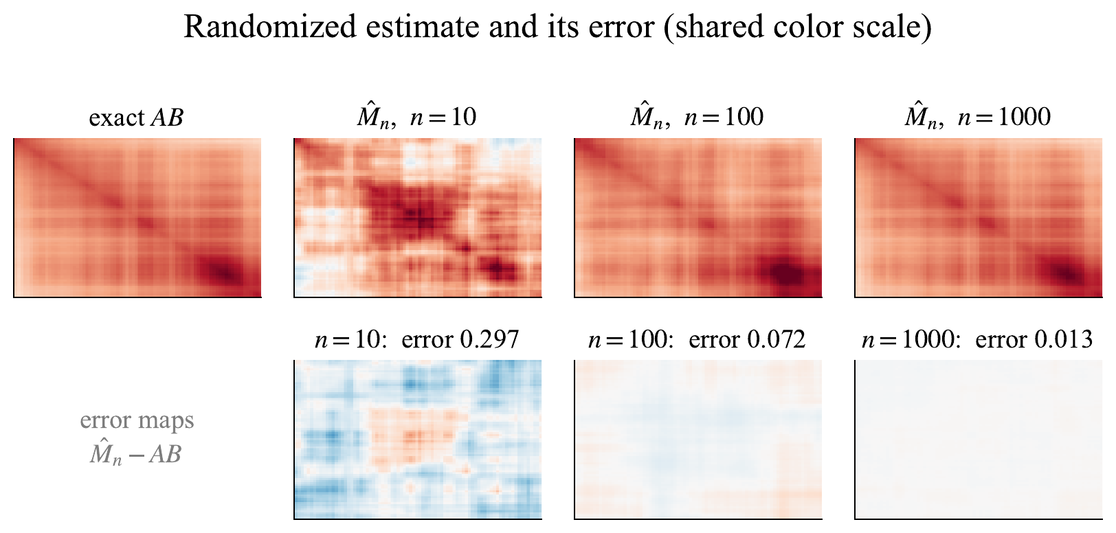
At \(n = 1000\) the estimate already reproduces \(\mathbf{A}\mathbf{B}\) closely, entry by entry.
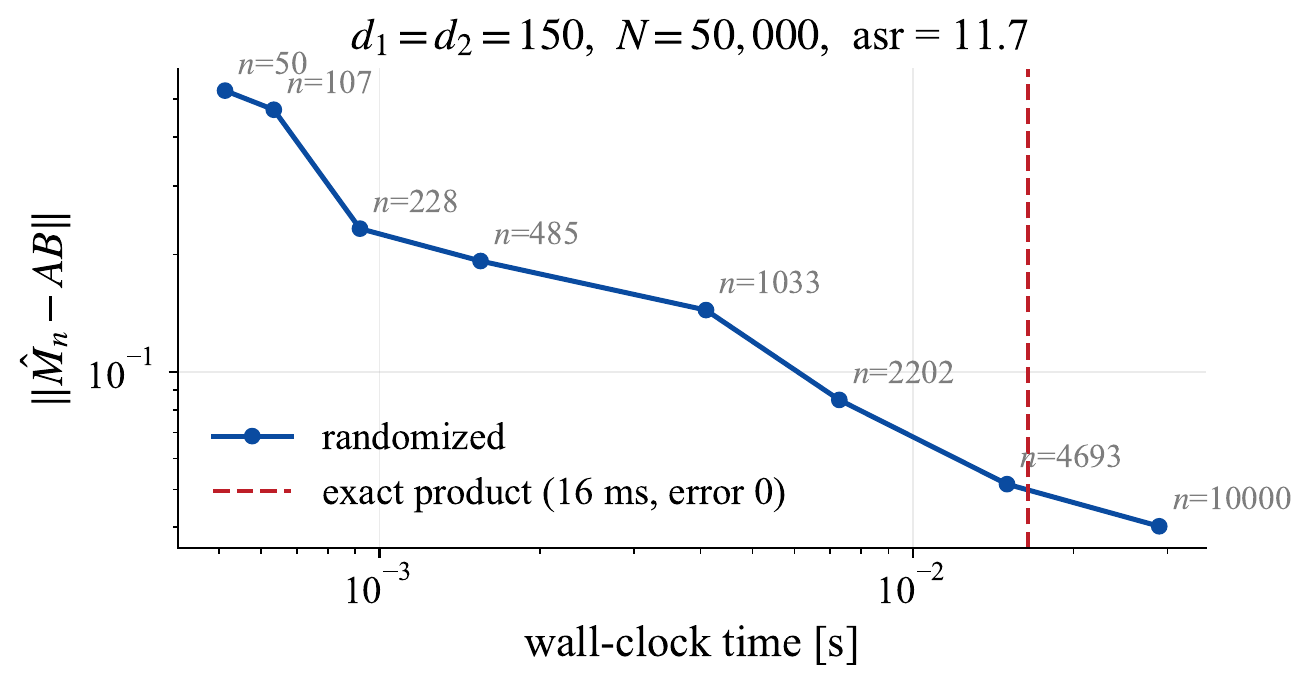
With \(N = 50\,000\), choosing \(n = 228\) (0.5% of the terms) runs about \(18\times\) faster at error \(0.23\).
5. Proof Ideas
The proof follows the scalar Chernoff recipe
\[\mathbb{P}\{S \geq t\} \leq e^{-\theta t} \prod_{k} \mathbb{E}[e^{\theta X_k}], \qquad \forall \theta > 0,\]but the product rule fails for matrices, since \(e^{\mathbf{A} + \mathbf{B}} \neq e^{\mathbf{A}} e^{\mathbf{B}}\) in general. The fix runs in four steps: a trace matrix moment generating function, subadditivity in place of the product rule, a moment bound per summand, and optimization over \(\theta\).
Step 1: Matrix Laplace transform
\[\mathbb{P}\{\lambda_{\max}(\mathbf{S}) \geq t\} \leq e^{-\theta t}\, \mathbb{E}\operatorname{Tr} e^{\theta \mathbf{S}}, \qquad \forall \theta > 0.\]The proof is as follows \(\begin{aligned} \mathbb{P}\{\lambda_{\max}(\mathbf{S}) \geq t\} &= \mathbb{P}\{e^{\theta \lambda_{\max}(\mathbf{S})} \geq e^{\theta t}\} && x \mapsto e^{\theta x} \text{ increasing} \\ &\leq e^{-\theta t}\, \mathbb{E}\big[e^{\theta \lambda_{\max}(\mathbf{S})}\big] && \text{Markov's inequality} \\ &= e^{-\theta t}\, \mathbb{E}\big[e^{\lambda_{\max}(\theta \mathbf{S})}\big] && \theta \lambda_{\max}(\mathbf{S}) = \lambda_{\max}(\theta \mathbf{S}) \\ &= e^{-\theta t}\, \mathbb{E}\big[\lambda_{\max}(e^{\theta \mathbf{S}})\big] && \text{spectral mapping} \\ &\leq e^{-\theta t}\, \mathbb{E}\big[\operatorname{Tr} e^{\theta \mathbf{S}}\big] && \lambda_{\max}(\mathbf{M}) \leq \operatorname{Tr}\mathbf{M},\ \mathbf{M} \succ 0 \end{aligned}\)
Bounding the trace in the other direction, \(\operatorname{Tr}\mathbf{M} \leq d\,\lambda_{\max}(\mathbf{M})\), is where the dimensional factor \(d\) enters the final result.
Step 2: Subadditivity
Lieb (1973). The map \(\mathbf{A} \mapsto \operatorname{Tr}\exp(\mathbf{H} + \log \mathbf{A})\) is concave on positive definite \(\mathbf{A}\).
Combined with Jensen’s inequality, this replaces the failed product rule:
\[\mathbb{E}\big[\operatorname{Tr} e^{\theta \mathbf{S}}\big] = \mathbb{E}\Big[\operatorname{Tr} e^{\theta \sum_{k=1}^n \mathbf{X}_k}\Big] \leq \operatorname{Tr} \exp\Big(\sum_{k=1}^{n} \log \mathbb{E}\big[e^{\theta \mathbf{X}_k}\big]\Big).\]Step 3: One summand at a time
For \(\mathbb{E}[\mathbf{X}] = \mathbf{0}\), \(\|\mathbf{X}\| \leq B\) and \(0 < \theta < 3/B\), a scalar bound plus the spectral theorem give
\[\log \mathbb{E}\big[e^{\theta \mathbf{X}}\big] \preccurlyeq \mathbb{E}\big[e^{\theta \mathbf{X}}\big] - \mathbf{I} \preccurlyeq g(\theta)\, \mathbb{E}[\mathbf{X}^2], \qquad g(\theta) = \frac{\theta^2/2}{1 - \theta B/3}.\]Only two features of each summand are used: the uniform bound \(B\) and the second moment \(\mathbb{E}[\mathbf{X}^2]\).
Step 4: Assemble and optimize
\[\mathbb{P}\{\lambda_{\max}(\mathbf{S}) \geq t\} \leq e^{-\theta t}\operatorname{Tr}\exp\Big(g(\theta) \sum_{k} \mathbb{E}[\mathbf{X}_k^2]\Big) \leq d\, e^{-\theta t} \exp\big(g(\theta) v\big).\]Choosing \(\theta_\star = t / (v + Bt/3)\) yields the stated inequality
\[\mathbb{P}\{\lambda_{\max}(\mathbf{S}) \geq t\} \leq d \exp\left(\frac{-t^2/2}{v + Bt/3}\right).\]Key Messages
- Matrix concentration gives non-asymptotic bounds, valid for every \(n\) and \(d\).
- One independent-sum model covers covariance estimation, empirical Hessians, and randomized matrix multiplication.
- The proof runs through the matrix moment generating function, with Lieb’s theorem replacing the scalar product rule.
Further reading. Tropp, J. A. (2015). An introduction to matrix concentration inequalities. Foundations and Trends in Machine Learning.